多変量正規分布の復習
\(x\)がK変量正規分布に従い、平均ベクトルを\(\mu\)、共分散行列を\(\Sigma\)とおくと、\(y\)の同時確率密度関数は以下のように表される。参考記事
\[MultiNormal(x|\mu,\Sigma) = \frac{1}{\left( 2 \pi \right)^{K/2}} \frac{1}{\sqrt{|\Sigma|}} \exp \! \left( \! - \frac{1}{2} (x - \mu)^{\top} \, \Sigma^{-1} \, (x - \mu) \right)\]
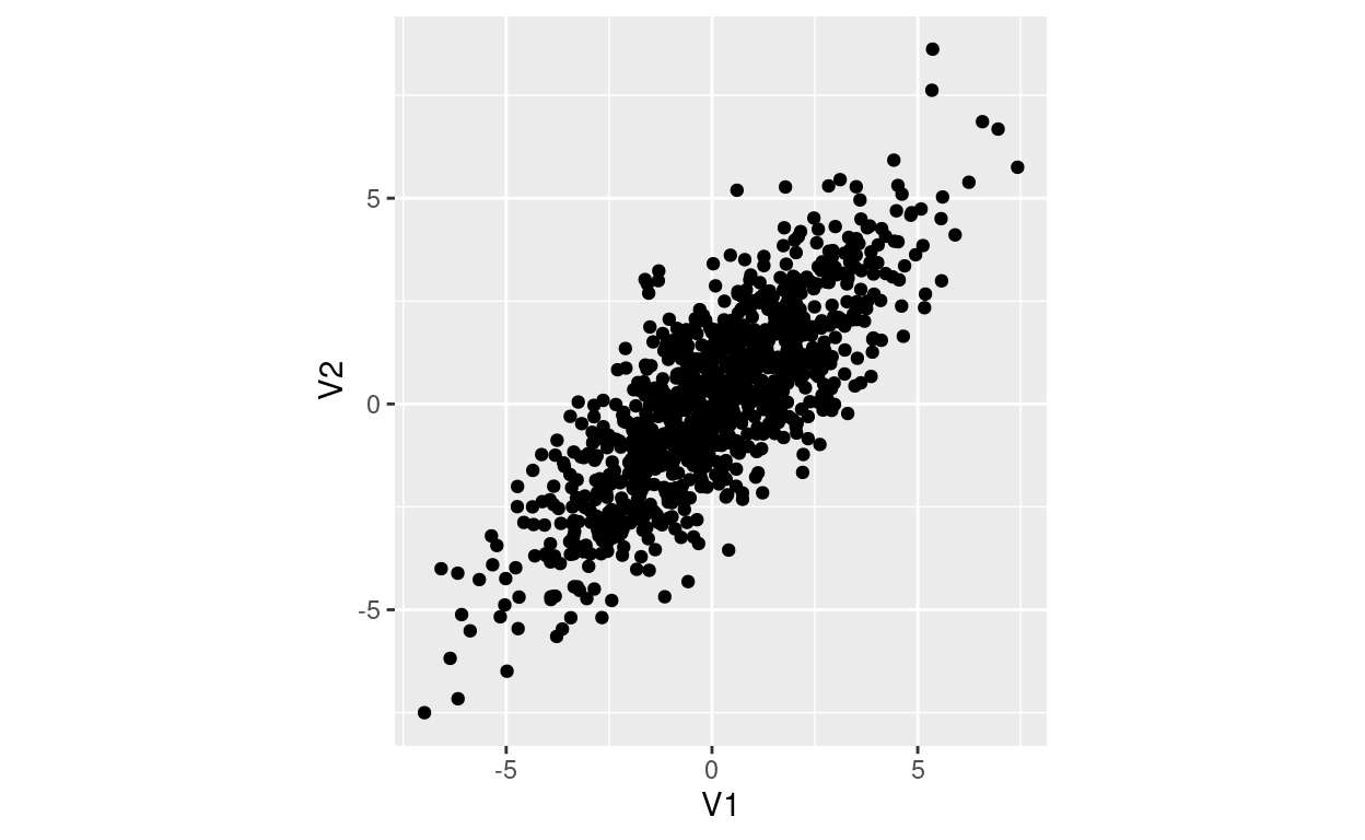
例のため、\(\mu = \textbf{0}\), \(\Sigma = \left[\begin{matrix} 5 & 4 \\ 4 & 5 \end{matrix}\right]\) とする。
可視化してみると、
library(tidyverse)
Sigma <- matrix(c(5, 4, 4, 5), nrow=2)
df <- MASS::mvrnorm(n=1000, mu=c(0, 0), Sigma=Sigma) %>% as_tibble()
ggplot(df, aes(V1, V2)) +
  geom_point() +
  coord_fixed() +
  scale_x_continuous(breaks = seq(-10, 10, 5)) +
  scale_y_continuous(breaks = seq(-10, 10, 5)) -> p
p
共分散行列の固有値、固有ベクトルを求める。
eigen(Sigma)
eigen() decomposition
$values
[1] 9 1

$vectors
          [,1]       [,2]
[1,] 0.7071068 -0.7071068
[2,] 0.7071068  0.7071068
固有値: \(\lambda = 9, 1\)
固有ベクトル: (0.7071068, 0.7071068), (-0.7071068, 0.7071068)
固有ベクトルはノルムが1に正規化されている。
固有ベクトルが軸の方向、固有値が楕円の大きさを示している。
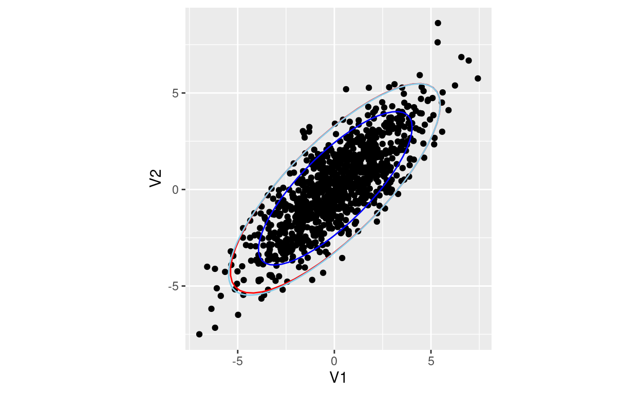
HDRの可視化
HDRについてはここを参照。
サンプルから推定された80%, 95% HDR (red, blue).
共分散行列から計算される95% HDR (skyblue). ここを参考にした。
c95 <- qchisq(.95, df=2)
ellips <- function(center = c(0,0), conf=c95, cov_mat, npoints = 100){
  t <- seq(0, 2*pi, len=npoints)
  #Sigma <- matrix(c(1, rho, rho, 1), 2, 2)
  Sigma <- cov_mat
  a <- sqrt(conf*eigen(Sigma)$values[2])
  b <- sqrt(conf*eigen(Sigma)$values[1])
  x <- center[1] + a*cos(t)
  y <- center[2] + b*sin(t)
  X <- cbind(x, y)
  R <- eigen(Sigma)$vectors
  data.frame(X%*%R)
}
dat <- ellips(center=c(0, 0), cov_mat=Sigma, c=c95, npoints=100)
p +
  stat_ellipse(type = "norm", level = 0.8, color = "blue") +
  stat_ellipse(type = "norm", level = 0.95, color = "red") +
  geom_path(data=dat, aes(x=X1, y=X2), colour='skyblue')
HDRに含まれるか判定
あるK変量正規分布に従う点 \(\textbf{x}\)がHDRに含まれるかはMahalanobis距離、すなわち
\[(x - \mu)^{\top} \, \Sigma^{-1} \, (x - \mu) \leq \chi^{2}_{0.95}(K) \] で判定できる。
df <- df %>%
  bind_cols(d = mahalanobis(df, center = c(0, 0), cov = Sigma)) %>%
  mutate(flag = if_else(d < c95, TRUE, FALSE))
ggplot(df, aes(V1, V2, color=flag)) +
  geom_point() +
  coord_fixed() +
  scale_x_continuous(breaks = seq(-10, 10, 5)) +
  scale_y_continuous(breaks = seq(-10, 10, 5)) +
  geom_path(data=dat, aes(x=X1, y=X2), colour='skyblue')
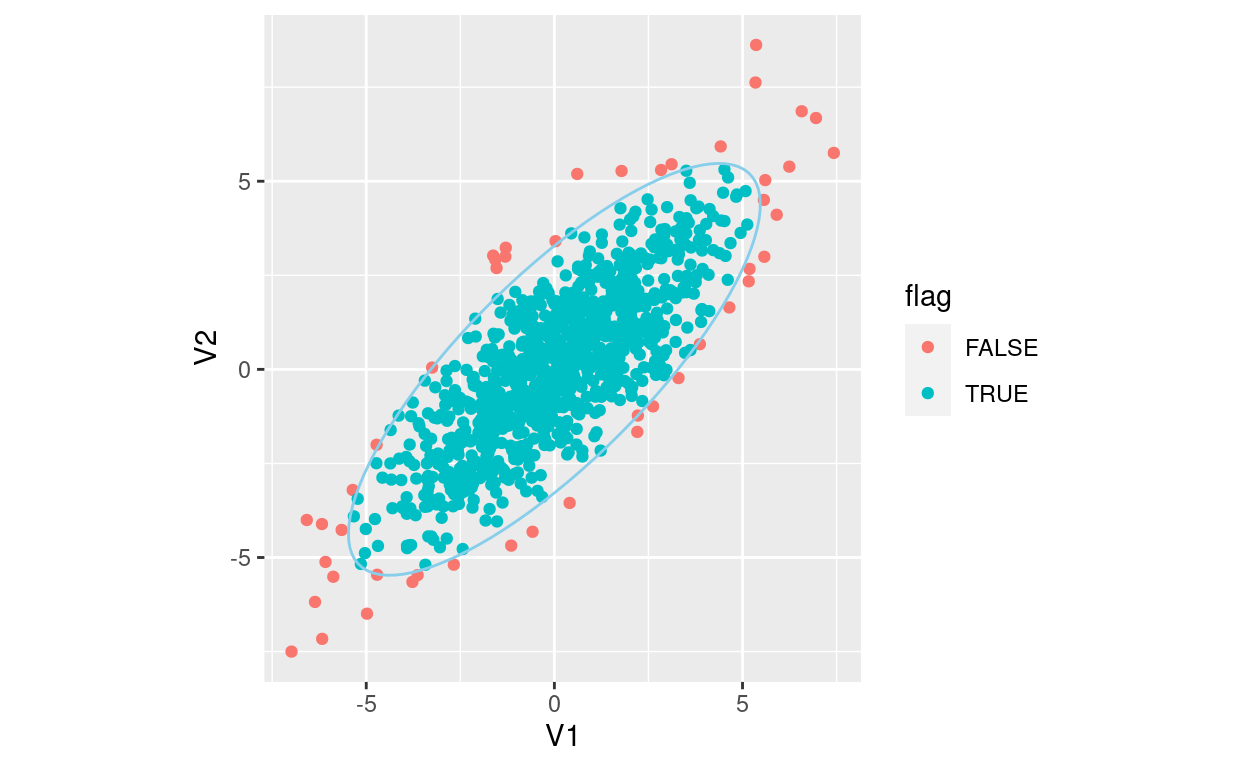
95%含まれているか確認
# A tibble: 2 × 3
  flag      n  freq
  <lgl> <int> <dbl>
1 FALSE    48 0.048
2 TRUE 952 0.952mahalanobisのソース
stats:::mahalanobis
function (x, center, cov, inverted = FALSE, ...)
{
    x <- if (is.vector(x))
        matrix(x, ncol = length(x))
    else as.matrix(x)
    if (!isFALSE(center))
        x <- sweep(x, 2L, center)
    if (!inverted)
        cov <- solve(cov, ...)
    setNames(rowSums(x %*% cov * x), rownames(x))
}
<bytecode: 0x555798789850>
<environment: namespace:stats>
その他参考